Google Sheets QUERY: Pivot Data
PIVOT
Thanks to PIVOT, it is possible to add new result columns from unique data in a column.
Example of Use
The following example displays the sum of messages (E) for each rank (D):
=QUERY(DB!A1:G15,"SELECT D, SUM(E) GROUP BY D")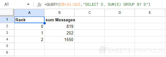
To display the ranks as a column (with one column per different rank) and the corresponding sum underneath, enter:
=QUERY(DB!A1:G15,"SELECT SUM(E) PIVOT D")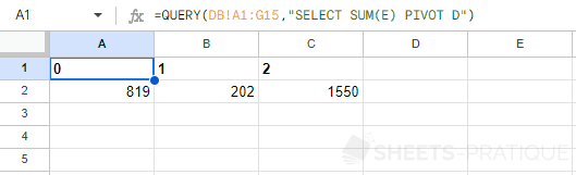
In this case, PIVOT pivoted the ranks to display one rank per column instead of displaying one rank per row.
It is also possible to modify the headers:
=QUERY(DB!A1:G15,"SELECT SUM(E) PIVOT D LABEL SUM(E) '(rank)'")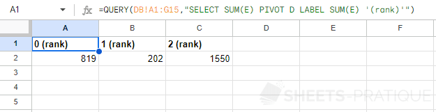
Advanced Use Case
The following example displays the sum of messages (E) for each rank (D):
=QUERY(DB!A1:G15,"SELECT D, SUM(E) GROUP BY D")The goal this time is to display the sum of messages for each rank (D) and for each month (B).
To achieve this result, one or the other of these data will therefore have to be pivoted.
To pivot based on ranks (D), enter:
=QUERY(DB!A1:G15,"SELECT MONTH(B), SUM(E) GROUP BY MONTH(B) PIVOT D")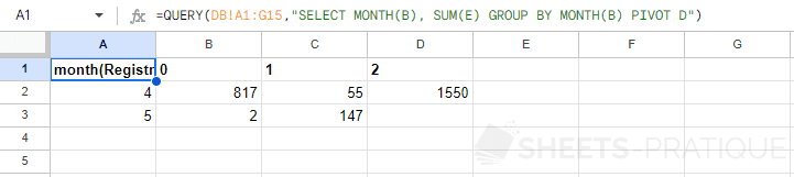
To pivot based on the months of dates (B), enter:
=QUERY(DB!A1:G15,"SELECT D, SUM(E) GROUP BY D PIVOT MONTH(B)")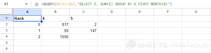
The same query with the addition of LABEL and FORMAT:
=QUERY(DB!A1:G15,"SELECT D, SUM(E) GROUP BY D PIVOT MONTH(B) LABEL SUM(E) '/ 2023', D '' FORMAT D 'Rank 0'")