Google Sheets Course: Tables (Formatting)
The objective of this new lesson is to understand how to apply a table-like formatting (borders, border styles, and background color).
Borders
Start by creating a new spreadsheet.
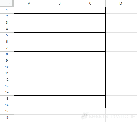
To apply borders to a range of cells, select it, click on then again on to apply borders on all sides:

You then get a first grid:
You may notice that there are different choices in this drop-down list. These icons tell you where the borders are applied.
Now erase this grid by clicking on :
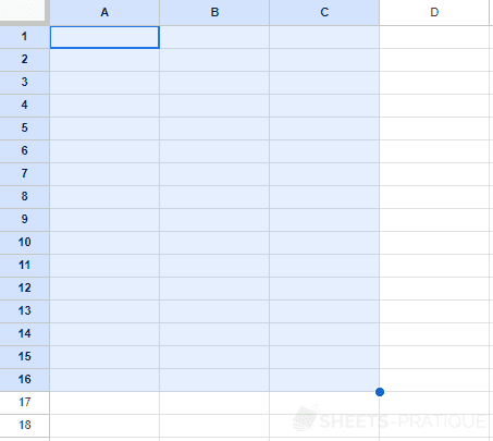
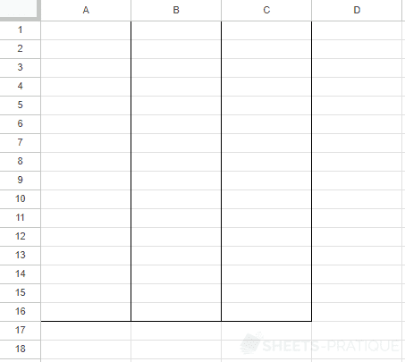
Keep this selection and apply borders inside the selection by clicking on :
Then apply borders around the selection by clicking on to get:
Border style
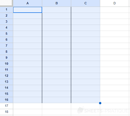
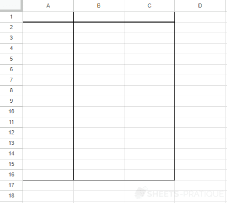
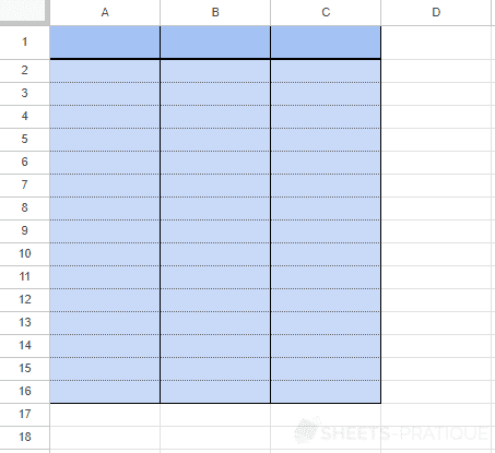
To apply a thicker border to the first row of the table, select cells from A1 to C1, modify the border style:

And apply the border with the chosen style by clicking on to target only the bottom border of the selection:
Border color
To change the color of a border, the principle is the same as changing the border style.
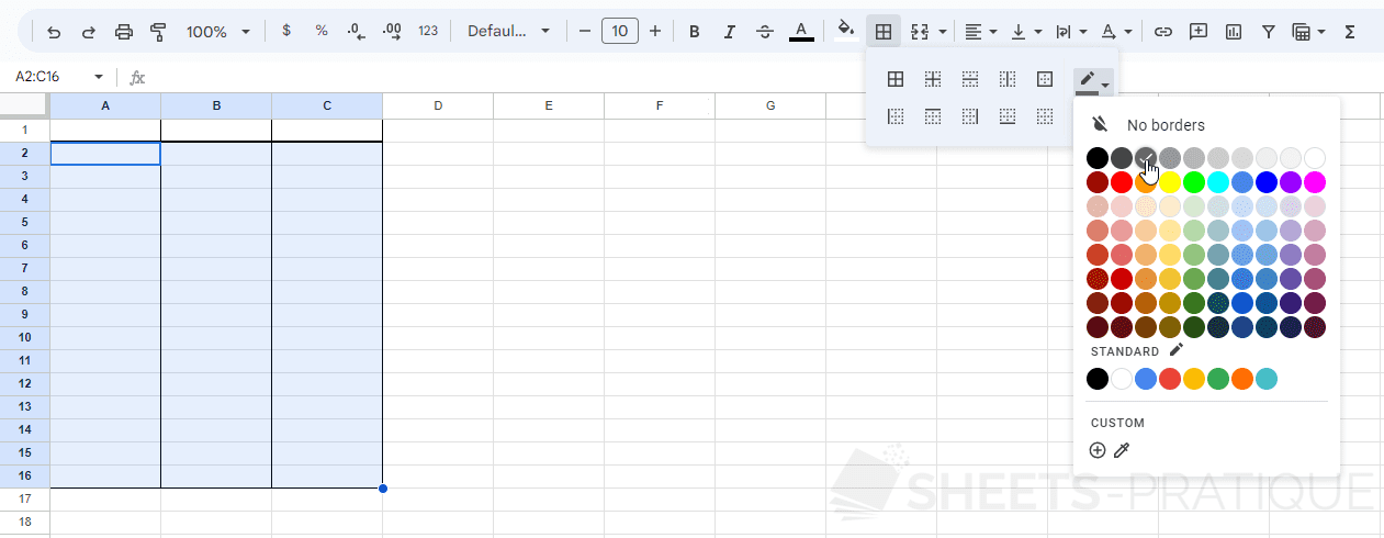
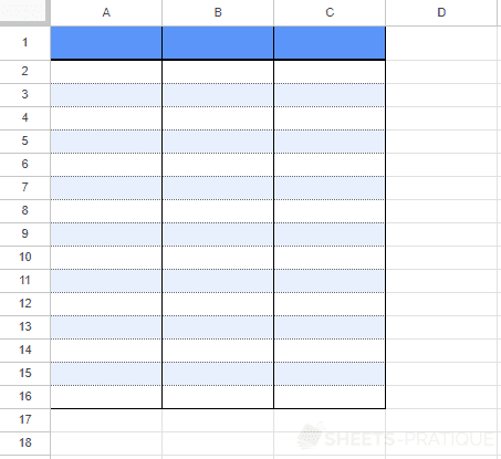
Now select the range of cells from A2 to C16 and choose the gray border color:
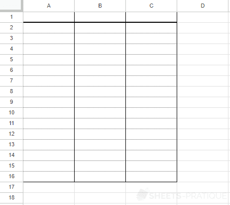
For this example, also change the border style to the dotted style and apply the borders horizontally and inside the selection by clicking on to get:
Background color
You can change the background colors and the line and column widths as you have already seen in the previous lesson:
A more practical solution is to select the entire table and then click on "Alternating colors":

Then choose one of the suggested styles or customize it:

Then validate your choice by clicking on Done.
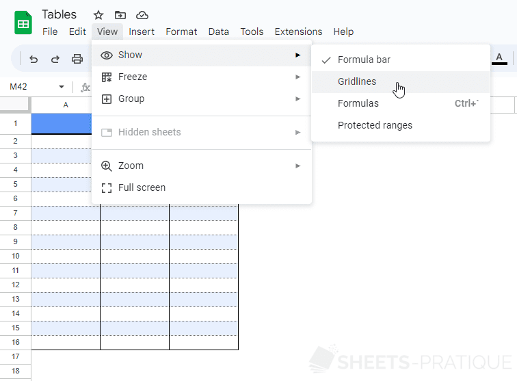
Hide the sheet grid
If you want to hide the cell grid displayed by default, uncheck "Gridlines" in the View menu: