Activate Conditional Formatting with a Checkbox
To activate conditional formatting in Google Sheets using a checkbox, use the AND function to add the reference of the checkbox cell.
Usage Example
In this example, a conditional formatting should display the top 5 highest amounts provided that the checkbox is checked:
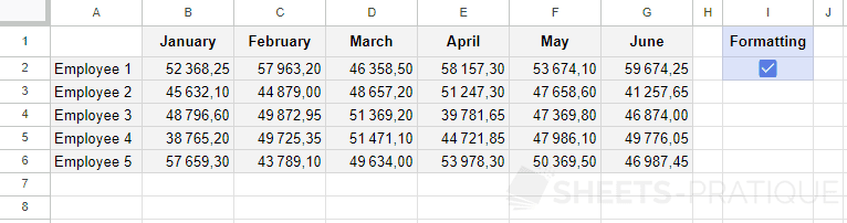
Start by selecting the cell range of the amounts, add a conditional formatting and choose the formatting rule "Custom formula is".
To check if an amount is among the top 5 in the range, the RANK function will be used here:
=RANK(B2,$B$2:$G$6,0)<=5
To activate this formatting only when the checkbox is checked, now add the formula of the conditional formatting in the AND function and the cell of the checkbox (with the $) as the second argument:
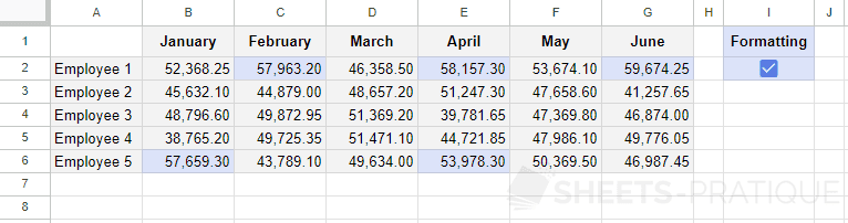
=AND(RANK(B2,$B$2:$G$6,0)<=5,$I$2)
Display when the checkbox is checked:
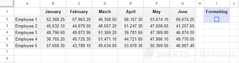
Display when the checkbox is unchecked:
If needed, you can copy the Google Sheets document (or view the document) with this example.