Google Sheets Course: IF Function and Nesting

Cell References

Instead of trying to display "Yes" and "No" depending on the age as is the case on the previous page, it is also possible to display a value contained in a cell.

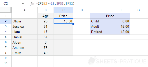
The goal is now to display a price depending on the age:

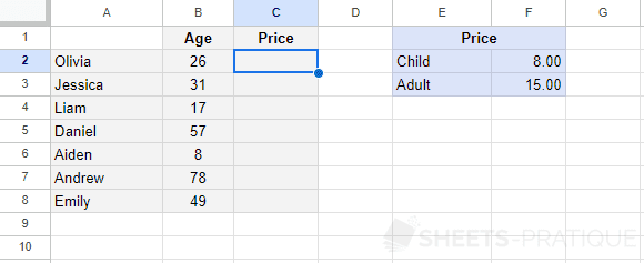
The texts "Yes" and "No" are therefore replaced by references to the prices:

=IF(B2>=18,F3,F2)

Do not forget to add $ to the price references to prevent them from shifting when copying them:

=IF(B2>=18,$F$3,$F$2)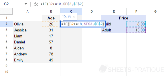

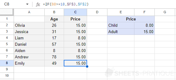
The prices are correctly displayed after copying:

Nesting a Function

In some cases, it will be necessary to nest several functions to achieve the desired result.

For example, if a third price is added:

In this case, if the person is 18 or older, 2 prices remain possible (adult and retired). A new IF condition must therefore be added to check if this person is retired or not and display the correct price.

To do this, instead of entering a reference to the adult price if the person is 18 or older, enter a new IF function:

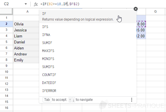
And complete this second IF function:

IF(B2<65,$F$3,$F$4)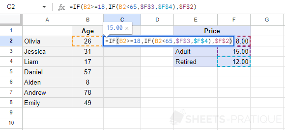

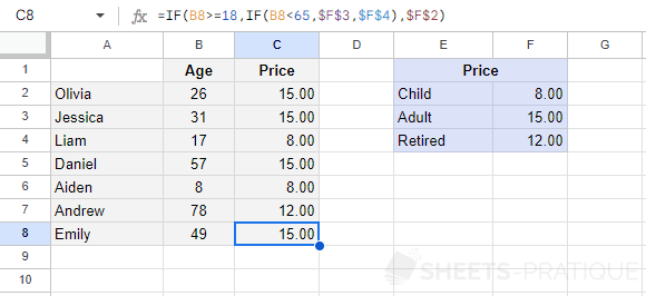
This formula containing 2 functions now allows displaying the 3 prices:

=IF(B2>=18,IF(B2<65,$F$3,$F$4),$F$2)