Google Sheets Function: SUMPRODUCT

The SUMPRODUCT function calculates the sum of products of two or more ranges of values multiplied together, row by row.

Usage:

=SUMPRODUCT(array1, array2)

or

=SUMPRODUCT(array1, array2, array3, ...)

Example of use

To better understand the SUMPRODUCT function and what "calculation of the sum of products" means, here is a simple table to start with:

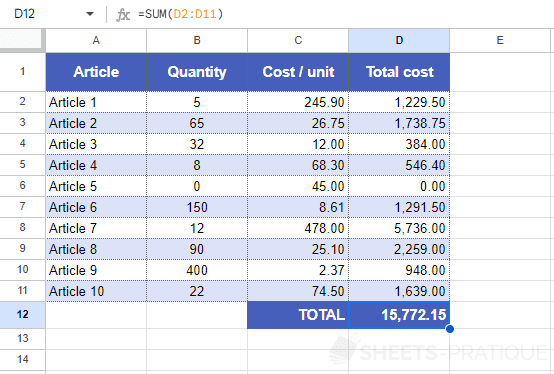
In this table, the total costs are the products of columns B and C =B2*C2, and the TOTAL is the sum of the various products =SUM(D2:D11).

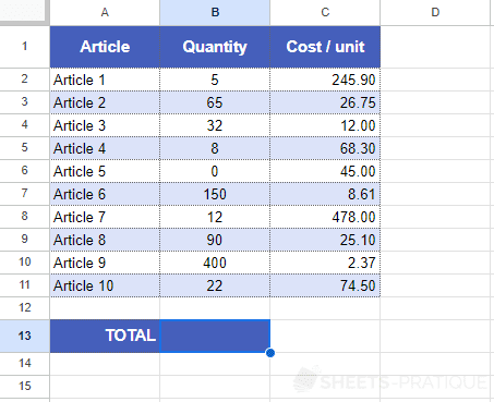
The goal now is to achieve the same result using SUMPRODUCT and without the total cost column:

Enter in the SUMPRODUCT function, the 2 cell ranges containing the data to multiply with each other (row by row) and for which you want to obtain the sum:

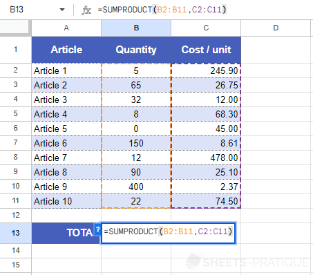
The following formula indeed returns the sum of products as in the first table:

=SUMPRODUCT(B2:B11,C2:C11)

Example of use with 3 ranges

By adding a third range, the SUMPRODUCT function will then return the sum of the products of the 3 ranges.

For example, by adding a column with checkboxes, only the rows with a checked box will be accounted for:

=SUMPRODUCT(B2:B11,C2:C11,D2:D11)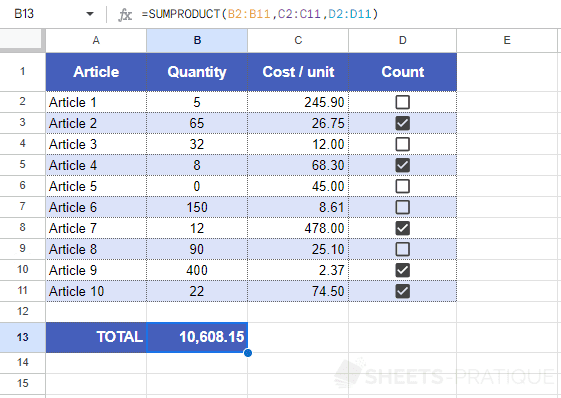

Example of use with a condition

To account for a range based on a condition (instead of checkboxes in the previous example), enter the range followed by the condition.

For example, to only account for rows where the quantity is greater than 100, enter:

=SUMPRODUCT(B2:B11,C2:C11,B2:B11>100)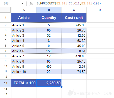

Just as with the checkboxes, this third range will return TRUE (= 1) or FALSE (= 0) depending on the condition >100, and will allow only the rows meeting this criteria to be counted.