Google Sheets Course: Custom Conditional Formatting

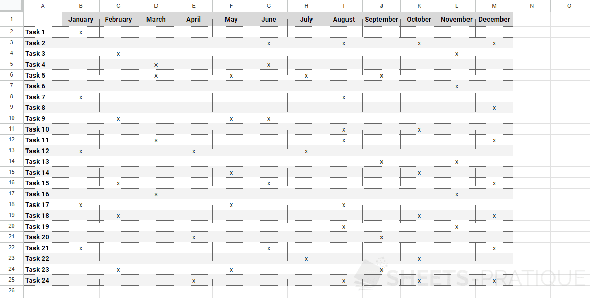
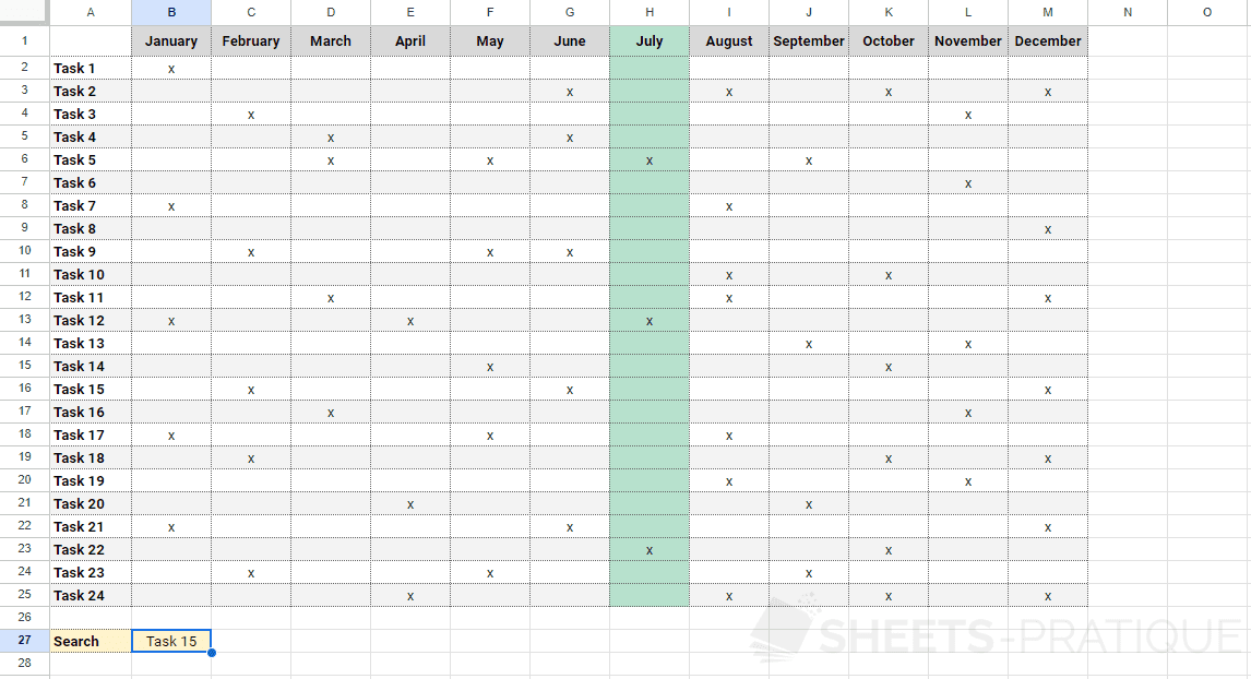
The goal of the custom conditional formatting will be here to color the column of the current month on the following schedule (lesson-9b.xlsx):

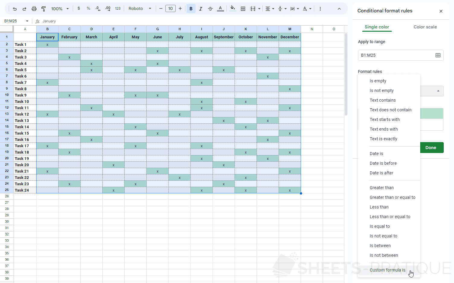
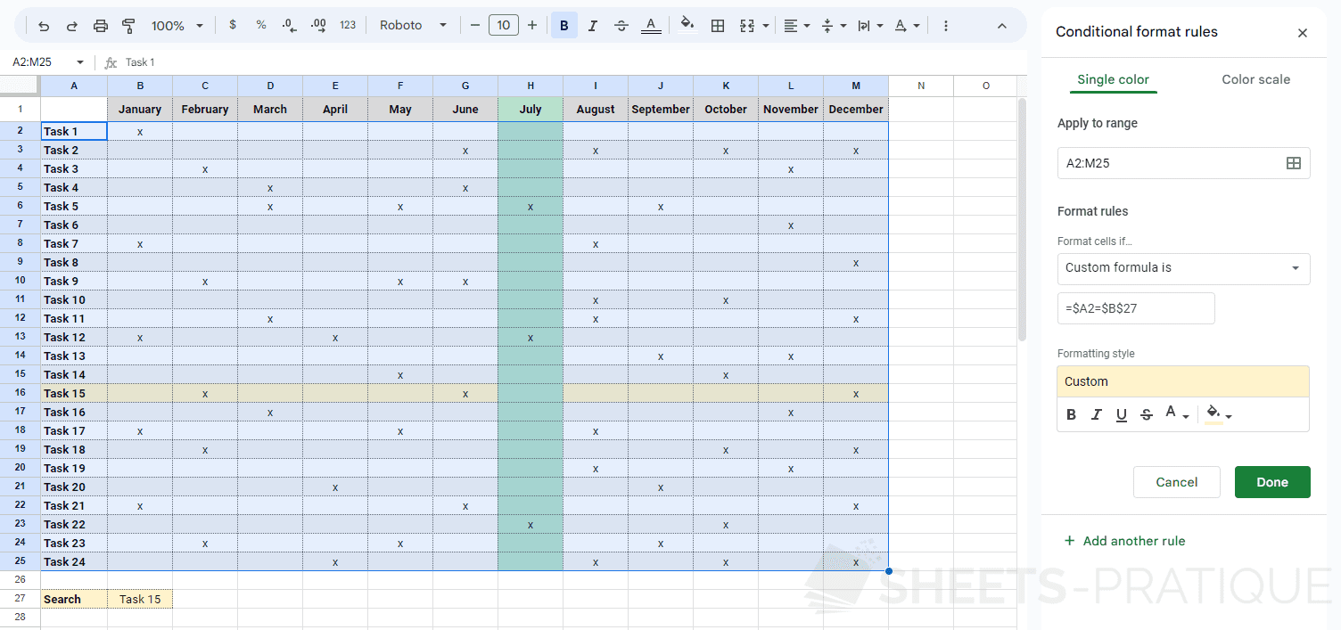
Select the range of cells concerned, add a "Conditional formatting" from the Format menu and choose the rule "Custom formula is":

The goal here is to format the entire column of the schedule according to the current month.

So we need to start by trying to know the current month.

The TODAY function returns the date of the day and the MONTH function returns the month of a date... The current month is therefore obtained thanks to MONTH(TODAY()).

We then need to determine which month each column corresponds to.

One solution is to use the COLUMN function which returns the current column number and to subtract 1 since the first month starts in column 2. The month of a column is therefore obtained thanks to COLUMN()-1.

The condition of the conditional formatting will then be COLUMN()-1=MONTH(TODAY()) which will return TRUE and trigger the formatting for the current month's column.

Since this is a formula, we still need to add an = at the beginning:

=COLUMN()-1=MONTH(TODAY())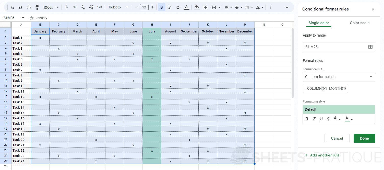

This example was created in July, so it is the month of July that is formatted on this image.

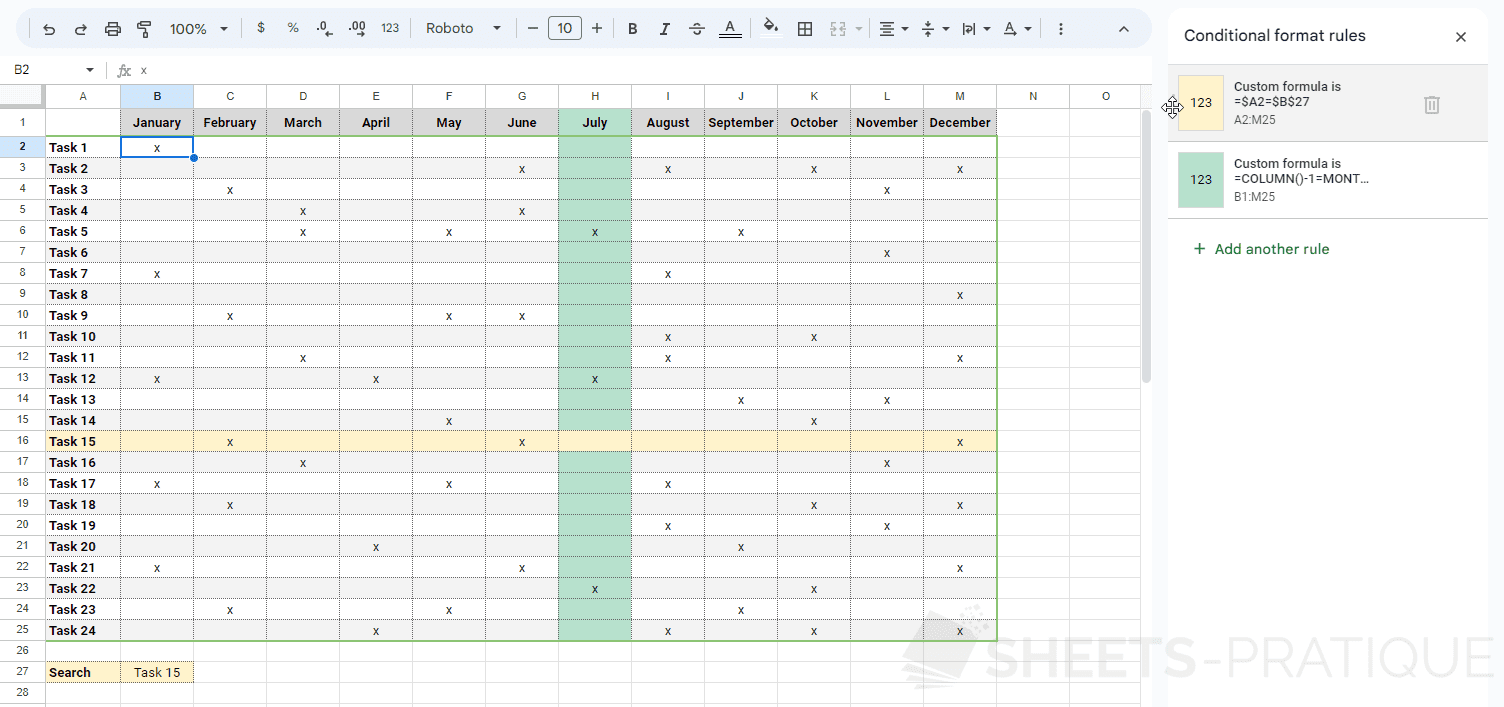
Now add the name of one of the tasks in cell B27:

This cell will serve as a search field for a second custom conditional formatting which will have to color the line of the table with an identical task name.

So you will simply need to check here if the cell to the left is equal to B27 A2=B27.

When you enter your formula, you must think of doing so for the cell in the top left of your selection. The formula will then adapt for the other cells as when you copy a formula (unless of course you have added $ to the references).

In this case, you will have to fix cell B27 which should not be shifted A2=$B$27.

In the formula, cell A2 will be able to be shifted by row but not by column (because the test will have to be performed on the first cell of each line for all the cells of the line), so you must only fix the column by adding a $ in front of the column $A2=$B$27:

You can then change the order of the conditional formats if needed: