Google Sheets Function: HLOOKUP

The HLOOKUP function searches for a value in the first row of a cell range and then returns the value of a cell in the same column.

Usage:

=HLOOKUP(search_key, range, index, is_sorted)

Example of use

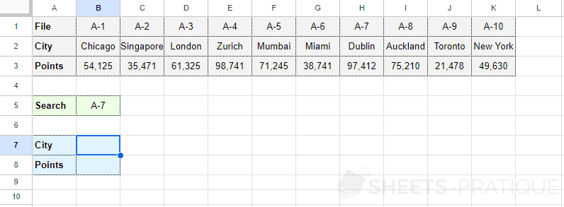
The objective here is to be able to enter the file number in cell B5 and then obtain the information for this file in the blue cells.

To start, the formula in cell B7 should return the name of the city:

Enter into the HLOOKUP function:

search_key: the value to search for in the first row of the range (here, the file number)
range: the range of cells containing all the data
index: the row number of the range that contains the result to return (here, row 2 for the city)
is_sorted: 0 to search for the exact value of search_key or 1 to return the closest value (provided the row is sorted), 0 is recommended in most cases

The formula here is:

=HLOOKUP(B5,B1:K3,2,0)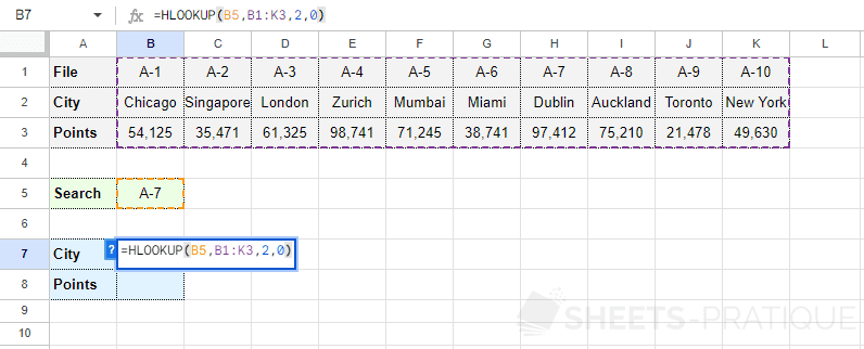

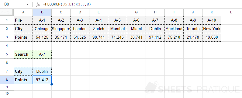
To then display the number of points, simply copy the formula and change the row number (replace 2 with 3):

If needed, you can copy the Google Sheets document (or view the document) with this example.

Since the HLOOKUP function searches for the value in the first row of the range, the results cannot be located above the search row. To perform a search in a row that is not necessarily the first of the range, use the XLOOKUP function.