Google Sheets Functions: INDEX + MATCH

The INDEX function used with the MATCH function allows for searching a value in a range of cells.

Prerequisites:

Before proceeding, please review the tutorial of the INDEX function and the MATCH function.

For a better understanding, the example proposed here is a combination of the examples from the 2 mentioned tutorials, and their reading is highly recommended.

INDEX + MATCH Functions

If the MATCH function returns a row number:

=INDEX(reference, MATCH(search_key, range, 0), column)

If the MATCH function returns a column number:

=INDEX(reference, row, MATCH(search_key, range, 0))

Example of use

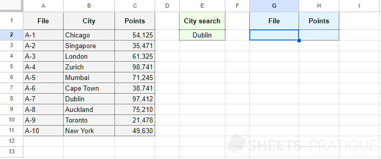
The objective here is to be able to enter the name of the city in cell E2 and then automatically obtain the desired information in the blue cells.

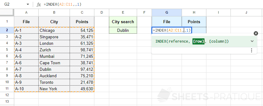
To start, the formula in cell G2 should return the file number of the searched city:

Enter into the INDEX function:

reference: the range of cells containing all the values
row: do not enter anything for now (the MATCH function that will determine the row number will be inserted here)
column: the column number of the value to return (in this case, the file number, so 1)

Then insert the MATCH function into "row" and complete the MATCH function:

search_key: the value whose position you wish to know (here, the city)
range: the range of cells in which the function will search for the position (here, the range of cells containing the cities)
search_type: 0 to find the exact value

The formula is therefore:

=INDEX(A2:C11,MATCH(E2,B2:B11,0),1)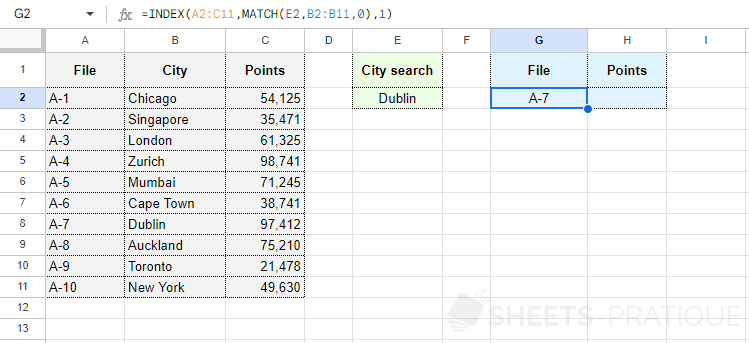

The file number of the searched city is now displayed.

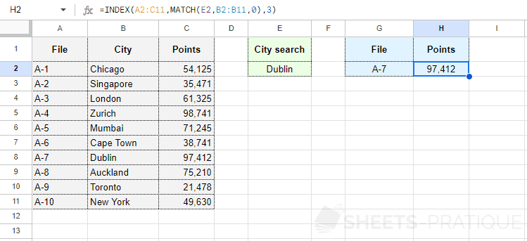
To then display the number of points of the city, simply copy the formula and change the column number (replace 1 with 3).

The second formula is:

=INDEX(A2:C11,MATCH(E2,B2:B11,0),3)

If needed, you can copy the Google Sheets document (or view the document) with this example.

Tip: It is generally simpler to use the XLOOKUP function for this type of search.