Google Sheets Function: XMATCH

The XMATCH function returns the position of a value in a range or an array.

This function is an enhanced version of the MATCH function.

Usage:

=XMATCH(search_key, lookup_range)

or

=XMATCH(search_key, lookup_range, match_mode, search_mode)

Example of use

The XMATCH function will here return the position of the searched city in the range of cities:

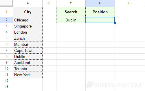
Enter into the XMATCH function:

• search_key: the value whose position you wish to know
• lookup_range: the range in which the function will search for the position of search_key

The formula here is:

=XMATCH(C2,A2:A11)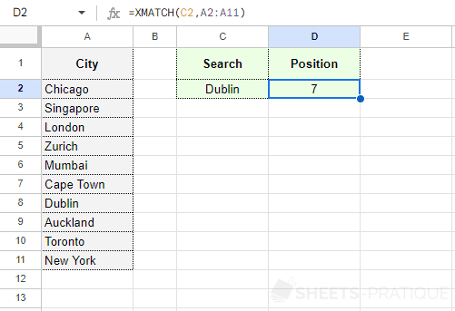

In this example, "Dublin" is indeed the seventh value in the range A2 to A11.

Optional Arguments

In the previous example, only the 2 mandatory arguments were specified, but there are 2 more optional ones:

• match_mode: the method for finding a match:
  • 0: exact match (default option)
  • 1: exact match or the next higher value to search_key
  • -1: exact match or the next lower value to search_key
  • 2: match with wildcard character
• search_mode: the search mode:
  • 1: search from the first entry to the last (default option)
  • -1: search from the last entry to the first
  • 2: binary search in the range assuming the range is sorted in ascending order
  • -2: binary search in the range assuming the range is sorted in descending order

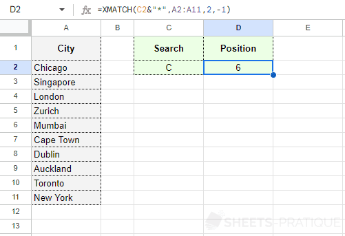
Here's another example using the wildcard character "*" (which replaces no, one, or multiple characters) and the search mode that starts from the end, to search for the position of a city that starts with "C" from the end:

=XMATCH(C2&"*",A2:A11,2,-1)