Google Sheets Function: INDEX

The INDEX function returns a value contained in a range based on a column and row number.

Usage:

=INDEX(reference, row, column)

Example of use

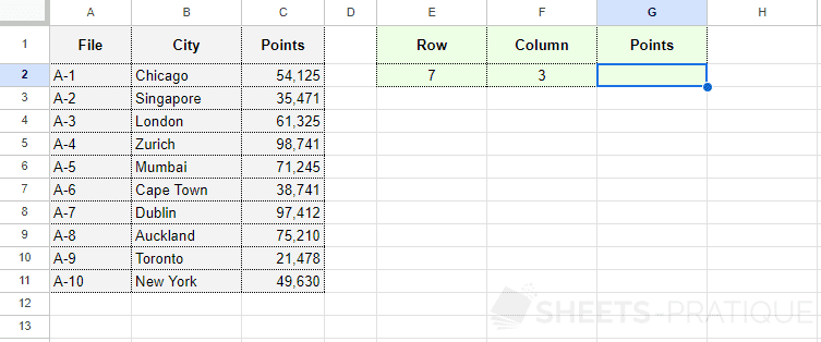
The objective here is to display a value from the range A2 to C11 based on the row and column numbers entered in cells E2 and F2:

Enter into the INDEX function:

• reference: the range of cells containing the values
• row: the row number of the value to return (in reference)
• column: the column number of the value to return (in reference)

The formula here is:

=INDEX(A2:C11,E2,F2)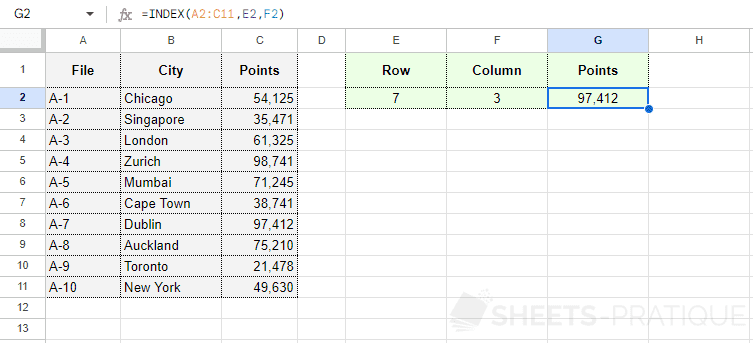

By combining this function with the MATCH function, it will then be possible to display the desired result based on a value in the table: INDEX + MATCH