Google Sheets Function: SUMIFS
The SUMIFS function allows for summing a range of cells based on multiple criteria (unlike the SUMIF function which is limited to a single criterion).
Usage:
=SUMIFS(sum_range, criteria_range1, criterion1)
or
=SUMIFS(sum_range, criteria_range1, criterion1, criteria_range2, criterion2, ...)
Usage Example
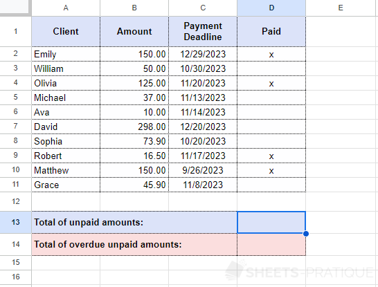
The SUMIFS function will be used here to first calculate the sum of unpaid amounts (= 1 criterion) and then the sum of overdue unpaid amounts (= 2 criteria):
Enter into the SUMIFS function:
- sum_range: the range of cells to be used for the sum calculation (here, the amounts)
- criteria_range1: the range of cells in which criterion1 will be checked (here, the "Paid" column)
- criterion1: the test
""to verify if the cell is empty
The formula is as follows:
=SUMIFS(B2:B11,D2:D11,"")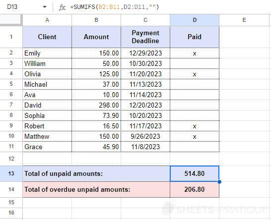
The SUMIF function could also have been used to perform this sum with a single condition (however, be aware that the order of arguments is not the same with this function).
To obtain the sum of overdue unpaid amounts, add a second criterion to the formula that checks if the payment deadline has passed (thus earlier than TODAY):
=SUMIFS(B2:B11,D2:D11,"",C2:C11,"<"&TODAY())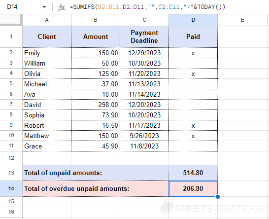
If needed, you can copy the Google Sheets document (or view the document) with this example.
Tip: it is possible to use wildcard characters with this function.